Using Scikit-learn’s Binary Trees to Efficiently Find Latitude and Longitude Neighbors

Engineering features from latitude and longitude data can seem like a messy task that may tempt novices into creating their own apply function (or even worse: an enormous for loop). However, these types of brute force approaches are potential pitfalls that will unravel quickly when the size of the dataset increases.

For example: Imagine you have a single dataset of n items. The time it takes to explicitly compare these n items against n-1 other items essentially approaches n². Meaning that with each doubling of rows in your dataset, the time it takes to find all nearest neighbors will increase by a factor of 4!

Fortunately, you do not need to calculate the distance between every point. There are a few data structures to efficiently determine neighbors right in scikit-learn that leverage the power of priority queues.

They can be found within the neighbors module and this guide will show you how to use two of these incredible classes to tackle this problem with ease.

Getting started

To begin we load the libraries.

import numpy as np
from sklearn.neighbors import BallTree, KDTree

# This guide uses Pandas for increased clarity, but these processes
# can be done just as easily using only scikit-learn and NumPy.
import pandas as pd

Then we’ll make two sample DataFrames based on weather station locations that are publicly available from the National Oceanic and Atmospheric Administration.

# Column names for the example DataFrame.
column_names = ["STATION NAME", "LAT", "LON"]

# A list of locations that will be used to construct the binary
# tree.
locations_a = [['BEAUFORT', 32.4, -80.633],
               ['CONWAY HORRY COUNTY AIRPORT', 33.828, -79.122],
               ['HUSTON/EXECUTIVE', 29.8, -95.9],
               ['ELIZABETHTON MUNI', 36.371, -82.173],
               ['JACK BARSTOW AIRPORT', 43.663, -84.261],
               ['MARLBORO CO JETPORT H E AVENT', 34.622, -79.734],
               ['SUMMERVILLE AIRPORT', 33.063, -80.279]]

# A list of locations that will be used to construct the queries.
# for neighbors.
locations_b = [['BOOMVANG HELIPORT / OIL PLATFORM', 27.35, -94.633],
               ['LEE COUNTY AIRPORT', 36.654, -83.218],
               ['ELLINGTON', 35.507, -86.804],
               ['LAWRENCEVILLE BRUNSWICK MUNI', 36.773, -77.794],
               ['PUTNAM CO', 39.63, -86.814]]

# Converting the lists to DataFrames. We will build the tree with
# the first and execute the query on the second.
locations_a = pd.DataFrame(locations_a, columns = column_names)
locations_b = pd.DataFrame(locations_b, columns = column_names)

This creates two DataFrames of a minuscule size: one with seven rows and one with four. For datasets this small, the data structures we are about to use will not offer any help in performance (and would actually be a hindrance). The documentation provides more information on when it would be more advantageous to choose one algorithm over another.

Using a k-d tree

We will start by demonstrating with a k-d tree. It will partition the datapoints into binary trees evaluating a single dimension at a time and splitting on the median. Then a query will be executed against it with another set of points and a value k to determine for each point how many neighbors you would like to return.

# Takes the first group's latitude and longitude values to construct
# the kd tree.
kd = KDTree(locations_a[["LAT", "LON"]].values, metric='euclidean')

# The amount of neighbors to return.
k = 2

# Executes a query with the second group. This will return two
# arrays.
distances, indices = kd.query(locations_b[["LAT", "LON"]], k = k)

The result is two arrays. One for the distances and one containing the indices of the neighboring locations (referring to the DataFrame that was used to construct the tree).

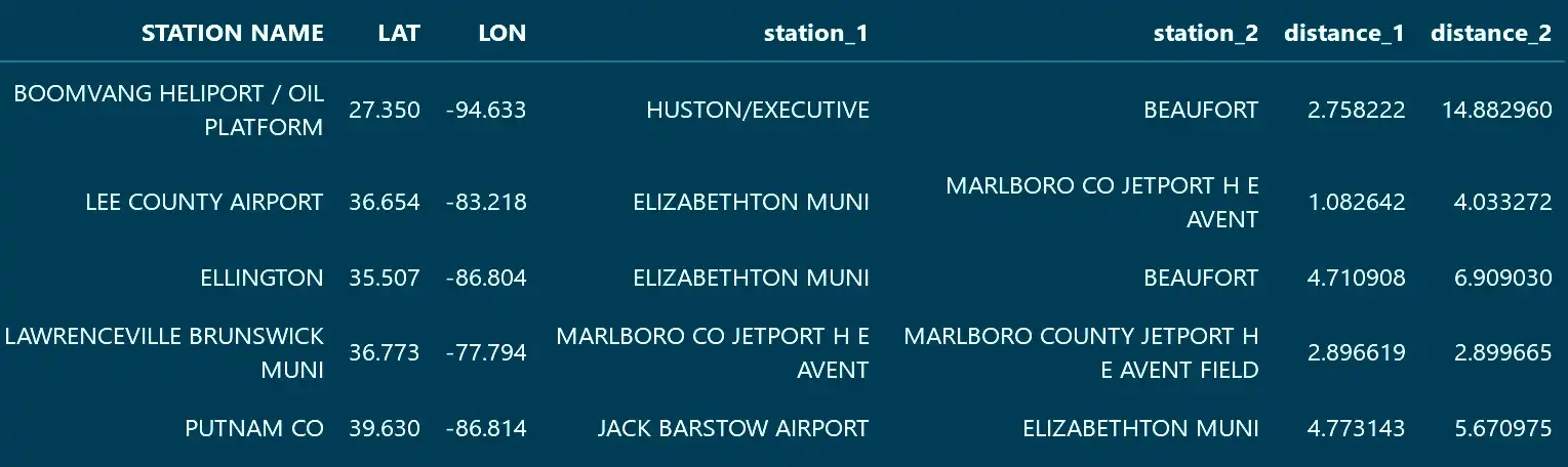
The indices can be then be mapped to useful values and both arrays easily merged with the rest of the data.

A few limitations

A k-d tree performs great in situations where there are not a large amount of dimensions. While this may seem fitting for the data here; in the case of latitude and longitude, evaluating based on differences in Euclidean distance will come with a cost in accuracy.

To more closely approximate the actual distance between coordinates we can use the Haversine distance. Unfortunately, the k-d tree algorithm will not work with this since it has a somewhat rigid approach in respect to each dimension. To see what available distance metrics can work with the k-d tree data structure, use this command:

KDTree.valid_metrics

Using a ball tree

A ball tree is similar to a k-d tree except that instead of making partitions across a single dimension, it will divide points based on radial distances to a center. It handles higher dimensional data better and will also permit the use of the Haversine metric.

To use a ball tree with the Haversine distance in scikit-learn, you must first convert the coordinates from degrees to radians.

# Creates new columns converting coordinate degrees to radians.
for column in locations_a[["LAT", "LON"]]:
    rad = np.deg2rad(locations_a[column].values)
    locations_a[f'{column}_rad'] = rad
for column in locations_b[["LAT", "LON"]]:
    rad = np.deg2rad(locations_b[column].values)
    locations_b[f'{column}_rad'] = rad

Aside from that, the two APIs are almost identical and most of the process will be repeated with minimal modifications.

# Takes the first group's latitude and longitude values to construct
# the ball tree.
ball = BallTree(locations_a[["LAT\_rad", "LON\_rad"]].values, metric='haversine')

# The amount of neighbors to return.
k = 2

# Executes a query with the second group. This will also return two
# arrays.
distances, indices = ball.query(locations_b[["LAT_rad", "LON_rad"]].values, k = k)

One final note: the distance returned will be based on the unit sphere with a radius of 1. If you’d like to see values that reflect typical measurements, it is an easy conversion.

• To miles: Distance x 3,958.8 (The radius of the earth in miles)
• To kilometers: Distance x 6,371 (The radius of the earth in kilometers)

With only 12 datapoints in this example, the advantage in using a ball tree with the Haversine metric cannot be shown. But in a larger dataset with less sparsity, it will be the choice you want to make when you are evaluating with latitude and longitude.

Of course, neither algorithm is limited to this use case alone and the steps shown here can be extended to any set of features that can be ordered by one of the many distance metrics.

The complex systems that we model have a myriad of influences contributing to the level of error that Data Scientists perpetually strive to reduce. With these tools at your disposal, you will be more equipped to efficiently discover additional factors and take feature engineering to a new level.